SDE simulation: creating synthetic datasets using SDEs

This example shows how to use numeric SDE solvers to simulate solutions of Stochastic Differential Equations (SDEs).

# Author: Pablo Soto Martín
# License: MIT
# sphinx_gallery_thumbnail_number = 2

SDEs represent a fundamental mathematical framework for modelling systems subject to both deterministic and random influences. They are a generalisation of ordinary differential equations, in which a diffusion or stochastic term is added. They are a great way of modelling phenomena with uncertain factors and are widely used in many scientific areas such us financial mathematics, quantum mechanics, engeneering, etc.

Mathematically, we can represent an SDE with the following formula:

\[d\mathbf{X}(t) = \mathbf{F}(t, \mathbf{X}(t))dt + \mathbf{G}(t, \mathbf{X}(t))d\mathbf{W}(t),\]

where \(\mathbf{X}\) is the vector-valued random variable we want to compute. The term \(\mathbf{F}\) is called the drift of the process, and the term \(\mathbf{G}\) the diffusion. The diffusion is a matrix which is multiplied by the vector \(\mathbf{W}(t)\), which represents a Wiener process.

To simulate SDEs practically, there exist various numerical integrators that approximate the solution with different degrees of precision. scikit-fda implements two of them: Euler-Maruyama and Milstein In this example we will use the Euler-Maruyama scheme due to its simplicity. However, the results can be reproduced also using Milstein scheme.

The example is divided into two parts:

• In the first part a simulation of trajectories is made.

• In the second part, the marginal probability flow of a stochastic process is visualized.

Simulation of trajectories of an Ornstein-Uhlenbeck process

Using numeric SDE solvers we can simulate the evolution of a stochastic process. One common SDE found in the literature is the Ornstein Uhlenbeck process (OU). The OU process is particularly useful for modelling phenomena where a system tends to return to a central value or equilibrium point over time, exhibiting a form of stochastic stability. In this case, the process can be modelled with the equation:

\[d\mathbf{X}(t) = -\mathbf{A}(\mathbf{X}(t) - \mathbf{\mu})dt + \mathbf{B} d\mathbf{W}(t)\]

where \(\mathbf{W}\) is the Brownian motion. The parameter \(\mu\) represents the equilibrium point of the process, \(\mathbf{A}\) represents the rate at which the process reverts to the mean and \(\mathbf{B}\) represents the volatility of the processs.

To illustrate the example, we will define some concrete values for the parameters:

from typing import Any

import numpy as np

NDArrayFloat = np.typing.NDArray[np.floating[Any]]

A = 1
mu = 3
B = 0.5


def ou_drift(
    t: float,
    x: NDArrayFloat,
) -> NDArrayFloat:
    """Drift of the Ornstein-Uhlenbeck process."""
    return -A * (x - mu)

For the first example, we will consider that all samples start from the same initial state \(X_0\). We can simulate the trajectories using the Euler - Maruyama method. The trajectories of the SDE calculated by skfda.datasets.make_sde_trajectories() are stored in an FDataGrid. Then, we can plot them using scikit-fda integrated functional data plots.

import matplotlib.pyplot as plt

from skfda.datasets import make_sde_trajectories

X_0 = 1.0

fd_ou = make_sde_trajectories(
    initial_condition=X_0,
    n_samples=30,
    drift=ou_drift,
    diffusion=B,
    start=0.0,
    stop=5.0,
    random_state=np.random.RandomState(1),
)

grid_points = fd_ou.grid_points[0]
fig = fd_ou.plot(alpha=0.8)
ax = fig.axes[0]
mean_ou = np.mean(fd_ou.data_matrix, axis=0)[:, 0]
std_ou = np.std(fd_ou.data_matrix, axis=0)[:, 0]
ax.fill_between(
    grid_points,
    mean_ou + 2 * std_ou,
    mean_ou - 2 * std_ou,
    alpha=0.25,
    color="gray",
)
ax.plot(
    grid_points,
    mean_ou,
    linewidth=2,
    color="k",
    label="empirical mean",
)
ax.plot(
    grid_points,
    mu * np.ones_like(grid_points),
    linewidth=2,
    label="stationary mean",
    color="b",
    linestyle="dashed",
)
ax.set_xlabel("t")
ax.set_ylabel("X(t)")
ax.set_title("Ornstein-Uhlenbeck simulation from an initial value")
ax.legend()
plt.show()

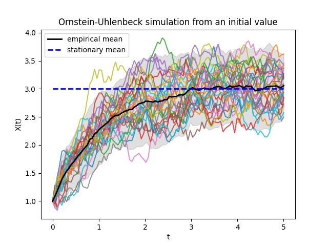
In the previous image we can observe 30 simulated trajectories. We can see how the empirical mean approaches the theoretical stationary mean of the process.

The initial point \(X_0\) from which we compute the simulation does not need to be always the same value. In the following code, we compute trajectories for the Ornstein-Uhlenbeck process for a range of initial points.

X_0 = np.linspace(1, 11, 30)

fd_ou = make_sde_trajectories(
    initial_condition=X_0,
    drift=ou_drift,
    diffusion=B,
    start=0.0,
    stop=5.0,
    random_state=np.random.RandomState(1),
)

grid_points = fd_ou.grid_points[0]
fig = fd_ou.plot(alpha=0.8)
ax = fig.axes[0]
mean_ou = np.mean(fd_ou.data_matrix, axis=0)[:, 0]
std_ou = np.std(fd_ou.data_matrix, axis=0)[:, 0]
ax.fill_between(
    grid_points,
    mean_ou + 2 * std_ou,
    mean_ou - 2 * std_ou,
    alpha=0.25,
    color="gray",
)
ax.plot(
    grid_points,
    mean_ou,
    linewidth=2,
    color="k",
    label="empirical mean",
)
ax.plot(
    grid_points,
    mu * np.ones_like(grid_points),
    linewidth=2,
    label="stationary mean",
    color="b",
    linestyle="dashed",
)
ax.set_xlabel("t")
ax.set_ylabel("X(t)")
ax.set_title("Ornstein-Uhlenbeck simulation from a range of initial values")
ax.legend()
plt.show()

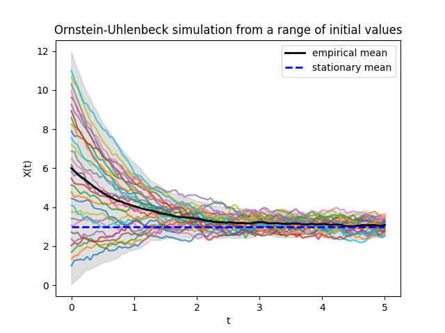
In the Ornstein-Uhlenbeck process, regardless the initial value, the trajectories tend towards the stationary distribution.

Probability flow

In this section we exemplify how to visualize the evolution of the marginal probability density, i.e. probability flow, of a stochastic differential equation. At a given time t, the solution of an SDE is not a real-valued vector; it is a random variable. Numeric integrators allow us to generate trajectories which represent samples of these random variables at a given time t. Probability flow is a very interesting characteristic to study when simulating SDE, as it gives us the possibility to visualiaze the probability distribution of the solution of the SDE at a given time. We will present a 1-dimensional and a 2-dimensional example.

In the first example, we will analyse the evolution of the Ornstein Uhlenbeck process defined above where all the trajectories start on the same value \(X_0\) (the initial distribution is a Dirac delta on \(X_0\)). The solution of the OU process is theoretically known, so we can compare it with the empirical data we get from numeric SDE integrators.

The theoretical marginal probability density of the process is given in the following function:

from scipy.stats import norm


def theoretical_pdf(
    t: float,
    x: NDArrayFloat,
    x_0: float = 0,
) -> NDArrayFloat:
    """Theoretical marginal pdf of an Ornstein-Uhlenbeck process."""
    mean = x_0 * np.exp(-A * t) + mu * (1 - np.exp(-A * t))
    std = B * np.sqrt((1 - np.exp(-2 * A * t)) / (2 * A))
    return norm.pdf(x, mean, std)

In this case we will simulate a big number of trajectories, so that we get better precision.

X_0 = 0.0
t_0 = 0.0
t_n = 3.0

fd = make_sde_trajectories(
    initial_condition=X_0,
    n_samples=5000,
    drift=ou_drift,
    diffusion=B,
    start=t_0,
    stop=t_n,
    random_state=np.random.RandomState(1),
)

We create an animation that compares the theoretical marginal density with a normalized histogram with the empirical data.

from matplotlib import rc
from matplotlib.animation import FuncAnimation

x_min, x_max = min(X_0 - 1, mu - 2 * B), max(X_0 + 1, mu + 2 * B)
x_range = np.linspace(x_min, x_max, 200)
epsilon_t = 1.0e-10  # Avoids evaluating singular pdf at t_0
times = np.linspace(t_0 + epsilon_t, t_n, 100)
fig, axes = plt.subplots(2, 1, figsize=(7, 10))
rc("animation", html="jshtml")

# Creation of the plot.
ax_trajectories = axes[0]
ax_distribution = axes[1]

ax_distribution.set_xlim(x_min, x_max)
ax_distribution.set_ylim(0, 4)
ax_distribution.set_xlabel("x")
ax_distribution.set_title("Distribution of X(t) = x | X(0) = 0")

ax_trajectories.set_xlim(t_0, t_n)
ax_trajectories.set_ylim(x_min, x_max)
lines_0 = ax_trajectories.plot(times[:1], fd.data_matrix[:30, :1, 0].T)
ax_trajectories.set_title(
    f"Ornstein Uhlenbeck evolution at time {round(times[0], 2)}",
)
ax_trajectories.set_xlabel("t")
ax_trajectories.set_ylabel("X(t)")

curve = ax_distribution.plot(
    x_range,
    theoretical_pdf(times[0], x_range),
    linewidth=4,
    label="Theoretical pdf",
    color="C1",
)

hist = None

def update(frame: int) -> None:
    """Creation of each frame of the animation."""
    global hist

    for i, line in enumerate(lines_0):
        line.set_data(times[:frame], fd.data_matrix[i, :frame, 0].T)
    ax.set_title(
        f"Ornstein Uhlenbeck evolution at time {round(times[frame], 2)}",
    )

    if hist:
        hist.remove()
    _, _, hist = ax_distribution.hist(
        fd.data_matrix[:, frame],
        bins=30,
        density=True,
        label="Empirical pdf",
        color="C0",
    )
    curve[0].set_data(x_range, theoretical_pdf(times[frame], x_range))
    ax_distribution.legend()


anim = FuncAnimation(fig, update, frames=range(100))
plt.close()
anim

Once Loop Reflect

In the second example, we visualize the probability flow of a 2-dimensional Ornstein Uhlenbeck process. This process has the same parameters than the previous 1-dimensional one in each coordinate. In this case, instead of starting all trajectories from the same value or range of values, the initial condition is a random variable. Note that at each time \(t\), the solution of the SDE \(\mathbf{X}(t)\) is a random variable. So, in the general case the initial condition of an SDE is a random variable. In order to simulate trajectories from an initial condition given my a random variable, first data will be sampled from the random variable and then used to calculate trajectories of the process. For this example, the distribution of the initial random variable is a 2d Gaussian mixture with three modes.

In this code we define the parameters of the Gaussian mixture, which will have three modes. We also define a function that enables us to sample from the distribution.

from scipy.stats import multivariate_normal

means = np.array([[-1, -1], [3, 2], [0, 2]])
cov_matrices = np.array(
    [[[0.4, 0], [0, 0.4]],
     [[0.5, 0], [0, 0.5]],
     [[0.2, 0], [0, 0.2]],
     ],
)
probabilities = np.array([0.3, 0.6, 0.1])


def rvs_gaussian_mixture(
    size: int,
    random_state: np.random.RandomState,
) -> NDArrayFloat:
    """Generate samples of a gaussian mixture."""
    n_gaussians, dim = np.shape(means)
    selected_gaussians = random_state.multinomial(size, probabilities)
    samples = [multivariate_normal.rvs(
        means[index],
        cov_matrices[index],
        random_state=random_state,
        size=selected_gaussians[index],
    ) for index in range(n_gaussians)
    ]

    samples = np.concatenate(samples)
    random_state.shuffle(samples)
    return np.array(samples)

Once we have defined an initial distribution and a way to sample from it, we generate trajectories using the Euler-Maruyama function.

random_state = np.random.RandomState(1)
A = np.array([1, 1])
mu = np.array([3, 3])
B = 0.5 * np.eye(2)

fd = make_sde_trajectories(
    initial_condition=rvs_gaussian_mixture,
    n_samples=500,
    drift=ou_drift,
    diffusion=B,
    stop=3,
    random_state=random_state,
)

We now create a 3d-plot in which we show the evolution of the marginal pdf of the samples. In order to calculate the empirical pdf, we use kernel density estimators.

from sklearn.neighbors import KernelDensity

x_range = np.linspace(-4, 6, 100)
y_range = np.linspace(-4, 6, 100)
x, y = np.meshgrid(x_range, y_range)

coords = np.column_stack((x.ravel(), y.ravel()))

fig3d = plt.figure(figsize=(7, 8))
ax_3d = fig3d.add_subplot(2, 1, 1, projection="3d")
ax = fig3d.add_subplot(2, 1, 2)
fig3d.suptitle("Kernel Density Estimation")

lims = (-4, 6)
cmap = "cividis"

ax_3d.set_xlim(*lims)
ax_3d.set_ylim(*lims)
ax_3d.set_zlim(0, 0.35)

ax_3d.set_xlabel("x")
ax_3d.set_ylabel("y")

ax.set_xlim(*lims)
ax.set_ylim(*lims)

surface = None
contour = None

kde = KernelDensity(bandwidth=0.5, kernel="gaussian")

def update3d(frame: int) -> None:
    """Creation of each frame of the 3d animation."""
    global surface
    global contour

    data = fd.data_matrix[:, frame, :]

    kde.fit(data)
    grid_points_3d = np.c_[x.ravel(), y.ravel()]
    z = np.exp(kde.score_samples(grid_points_3d))
    z = z.reshape(x.shape)

    if surface:
        surface.remove()
    surface = ax_3d.plot_surface(
        x,
        y,
        z,
        cmap=cmap,
        lw=0.2,
        rstride=5,
        cstride=5,
    )

    if contour:
        contour.remove()
    contour = ax.contourf(x, y, z, levels=25, cmap=cmap)


ani3d = FuncAnimation(fig3d, update3d, frames=range(100))
plt.close()
ani3d

Once Loop Reflect

Using Milstein’s method to compute SDE solutions

Apart from the default Euler-Maruyana scheme, scikit-fda also implements the Milstein scheme, a numerical SDE integrator of a higher order of convergence than the Euler-Maruyama scheme. When computing solution trajectories of an SDE, the Milstein method adds a term which depends on the spacial derivative of the diffusion term of the SDE (derivative with respect to \(\mathbf{X}\)). In the Ornstein-Uhlenbeck process, as the diffusion does not depend on the value of \(\mathbf{X}\), then both methods Euler Maruyama and Milstein are equivalent. In this section we show how to use the former function for SDEs where the diffusion term does depend on \(X\).

We will simulate a Geometric Brownian Motion (GBM). One of its notable applications is in modelling stock prices in financial markets, as it forms the basis for models like the Black-Scholes option pricing model. The SDE of a 1-dimensional GBM is given by the formula

\[dX(t) = \mu X(t) dt + \sigma X(t) dW(t),\]

where \(\mu\) and \(\sigma\) have constant values. To illustrate the example, we will define some concrete values for the parameters:

mu = 2
sigma = 1


def gbm_drift(t: float, x: NDArrayFloat) -> NDArrayFloat:
    """Drift term of a Geometric Brownian Motion."""
    return mu * x


def gbm_diffusion(t: float, x: NDArrayFloat) -> NDArrayFloat:
    """Diffusion term of a Geometric Brownian Motion."""
    return sigma * x


def gbm_diffusion_derivative(t: float, x: NDArrayFloat) -> NDArrayFloat:
    """Spacial derviative of the diffusion term of a GBM."""
    return sigma * np.ones_like(x)[:, :, np.newaxis]

When defining the derivative of the diffusion function, it is important to return an array that has one additional dimension compared to the original diffusion function. This is because the derivative of a function provides information about the rate of change in multiple directions, which requires an extra dimension to capture the changes along each axis.

We will simulate all trajectories from the same initial value \(X_0 = 1\).

X0 = 1
n_simulations = 500
n_steps = 100
n_l0_discretization_points = 5
random_state = np.random.RandomState(1)

fd = make_sde_trajectories(
    initial_condition=X0,
    n_samples=n_simulations,
    n_grid_points=n_steps,
    drift=gbm_drift,
    diffusion=gbm_diffusion,
    diffusion_derivative=gbm_diffusion_derivative,
    method="milstein",
    random_state=random_state,
)

grid_points = fd.grid_points[0]
fig = fd.plot(alpha=0.85)
ax = fig.axes[0]
std_gbm = np.std(fd.data_matrix, axis=0)[:, 0]
mean_gbm = np.mean(fd.data_matrix, axis=0)[:, 0]
ax.fill_between(
    grid_points,
    mean_gbm + 2 * std_gbm,
    mean_gbm - 2 * std_gbm,
    alpha=0.25,
    color="gray",
)
ax.plot(
    grid_points,
    mean_gbm,
    linewidth=2,
    color="k",
    label="empirical mean",
)
ax.plot(
    grid_points,
    np.exp(grid_points * mu),
    linewidth=2,
    label="theoretical mean",
    color="b",
    linestyle="dashed",
)
ax.set_xlabel("t")
ax.set_ylabel("X(t)")
ax.set_title("Geometric Brownian motion simulation")
ax.legend()
plt.show()