Shift Registration

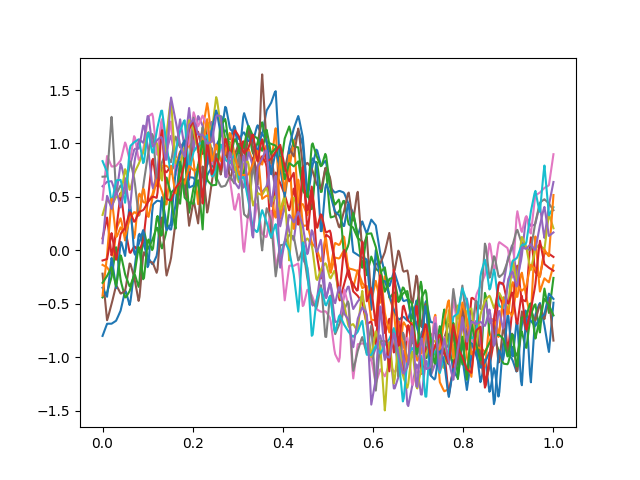
Shows the use of shift registration applied to a sinusoidal process represented in a Fourier basis.

# Author: Pablo Marcos Manchón
# License: MIT

# sphinx_gallery_thumbnail_number = 3

In this example we will use a sinusoidal process synthetically generated. This dataset consists in a sinusoidal wave with fixed period which contanis phase and amplitude variation with gaussian noise.

In this example we want to register the curves using a translation and remove the phase variation to perform further analysis.

import matplotlib.pyplot as plt

from skfda.datasets import make_sinusoidal_process

fd = make_sinusoidal_process(random_state=1)
fd.plot()
plt.show()

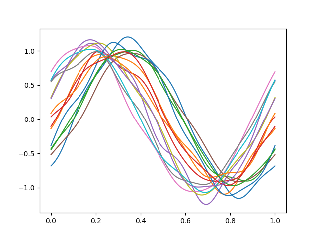
We will smooth the curves using a basis representation, which will help us to remove the gaussian noise. Smoothing before registration is essential due to the use of derivatives in the optimization process. Because of their sinusoidal nature we will use a Fourier basis.

from skfda.representation.basis import FourierBasis

fd_basis = fd.to_basis(FourierBasis(n_basis=11))
fd_basis.plot()
plt.show()

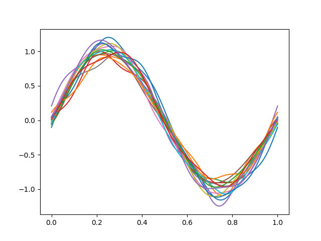
We will use the LeastSquaresShiftRegistration() transformer, which is suitable due to the periodicity of the dataset and the small amount of amplitude variation.

We can observe how the sinusoidal pattern is easily distinguishable once the alignment has been made.

from skfda.preprocessing.registration import LeastSquaresShiftRegistration


shift_registration = LeastSquaresShiftRegistration()
fd_registered = shift_registration.fit_transform(fd_basis)

fd_registered.plot()
plt.show()

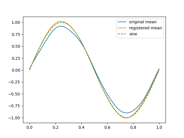
We will plot the mean of the original smoothed curves and the registered ones, and we will compare with the original sinusoidal process without noise.

We can see how the phase variation affects to the mean of the original curves varying their amplitude with respect to the original process, however, this effect is mitigated after the registration.

# sinusoidal process without variation and noise
sine = make_sinusoidal_process(
    n_samples=1,
    phase_std=0,
    amplitude_std=0,
    error_std=0,
)

fig = fd_basis.mean().plot()
fd_registered.mean().plot(fig)
sine.plot(fig, linestyle="dashed")

fig.axes[0].legend(["original mean", "registered mean", "sine"])
plt.show()

The values of the shifts \(\delta_i\), stored in the attribute deltas_ may be relevant for further analysis, as they may be considered as nuisance or random effects.

print(shift_registration.deltas_)

[ 0.09004943  0.01808744  0.08732826 -0.00013559 -0.04950421  0.11984576
 -0.09723283 -0.09330286 -0.04398832 -0.08389279  0.0583045   0.00503724
  0.08788296  0.0214795  -0.042531  ]