Mixed data structure and visualization.

This example demonstrates how to build and visualize mixed datasets containing both scalar and functional elements using the Canadian weather dataset. In particular, we show how to include both a function and its derivative, either jointly in a vector-valued functional object, or separately as independent entries. We also explore how to structure and visualize this data using pandas and scikit-fda’s visualization tools.

# Author: Luis Hebrero Garicano
# License: MIT
# sphinx_gallery_thumbnail_number = 1

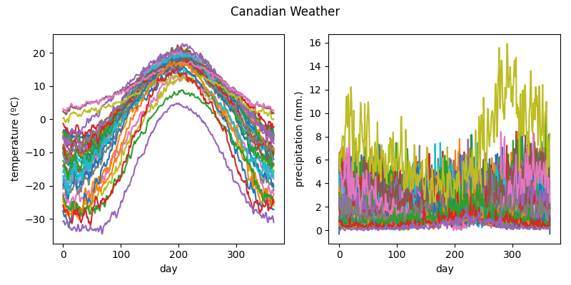
We load the Canadian weather dataset. This dataset includes daily temperature and precipitation curves for 35 weather stations in Canada, along with a scalar variable: the climate zone of each station.

from skfda import datasets

X, y = datasets.fetch_weather(return_X_y=True, as_frame=True)
fd = X.iloc[:, 0].values
fd_temperatures = fd.coordinates[0]
fd_precipitations = fd.coordinates[1]

We visualize the two functional components separately.

import matplotlib.pyplot as plt

fig, axes = plt.subplots(1, 2, figsize=(8, 4))

fd_temperatures.plot(axes=axes[0])
fd_precipitations.plot(axes=axes[1])
fig.tight_layout()
plt.show()

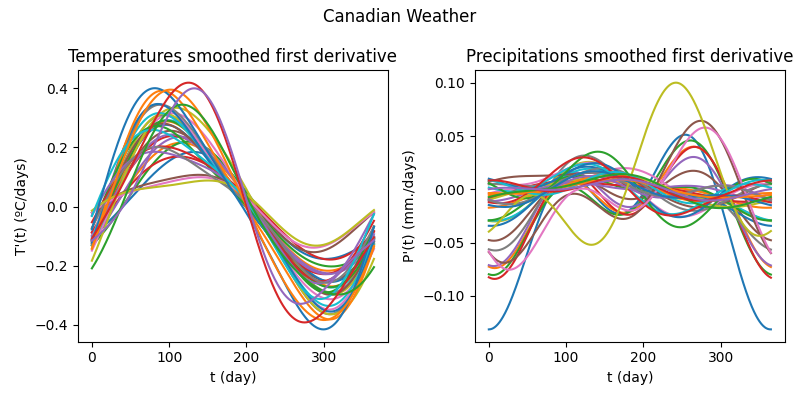
To enrich the data with information about temporal changes, we compute the first derivative of both temperature and precipitation curves. These derivatives can capture local variation patterns such as rising or falling trends.

fd_1st_temperatures = fd_temperatures.derivative()
fd_1st_precipitations = fd_precipitations.derivative()

Derivative curves often benefit from smoothing, especially when we plan to use them in downstream tasks like clustering or regression. We use Fourier basis representations with 5 elements for this purpose.

import skfda
from skfda.preprocessing.smoothing import BasisSmoother

range_temperatures = (
    fd_temperatures.grid_points[0][0],
    fd_temperatures.grid_points[0][-1],
)
range_precipitations = (
    fd_precipitations.grid_points[0][0],
    fd_precipitations.grid_points[0][-1],
)

basis_temperatures = skfda.representation.basis.FourierBasis(
    range_temperatures,
    n_basis=5,
)
basis_precipitations = skfda.representation.basis.FourierBasis(
    range_precipitations,
    n_basis=5,
)

smoother_temperatures = BasisSmoother(basis=basis_temperatures)
smoother_precipitations = BasisSmoother(basis=basis_precipitations)


fd_1st_temperatures_smooth = smoother_temperatures.fit_transform(
    fd_1st_temperatures,
)
fd_1st_precipitations_smooth = smoother_precipitations.fit_transform(
    fd_1st_precipitations,
)

fd_precipitations.argument_names = ("t (day)",)
fd_1st_precipitations_smooth.argument_names = ("t (day)",)
fd_1st_temperatures_smooth.argument_names = ("t (day)",)

fd_precipitations.coordinate_names = ("P(t) (mm.)",)
fd_1st_precipitations_smooth.coordinate_names = ("P'(t) (mm./days)",)
fd_temperatures.coordinate_names = ("T(t) (ºC)",)
fd_1st_temperatures_smooth.coordinate_names = ("T'(t) (ºC/days)",)

Let’s take a look at the smoothed derivatives.

fig, axes = plt.subplots(1, 2, figsize=(8, 4))

axes[0].set_title("Temperatures smoothed first derivative")
axes[1].set_title("Precipitations smoothed first derivative")

fd_1st_temperatures_smooth.plot(axes=axes[0])
fd_1st_precipitations_smooth.plot(axes=axes[1])

fig.tight_layout()
plt.show()

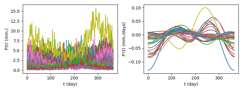
Now we build a vector-valued functional object that combines the original temperature and its derivative. This type of structure is useful when you want to treat them as a single feature with multiple components.

import numpy as np

from skfda.representation.grid import FDataGrid

data_matrix = np.concatenate(
    [fd_precipitations.data_matrix, fd_1st_precipitations_smooth.data_matrix],
    axis=2,
)

fd_vector = FDataGrid(
    data_matrix=data_matrix,
    grid_points=fd_temperatures.grid_points,
    coordinate_names=fd_precipitations.coordinate_names
    + fd_1st_precipitations_smooth.coordinate_names,
    argument_names=fd_1st_precipitations_smooth.argument_names,
)

fig, axes = plt.subplots(1, 2, figsize=(8, 3))

fd_vector.plot(axes=axes)
fig.tight_layout()
plt.show()

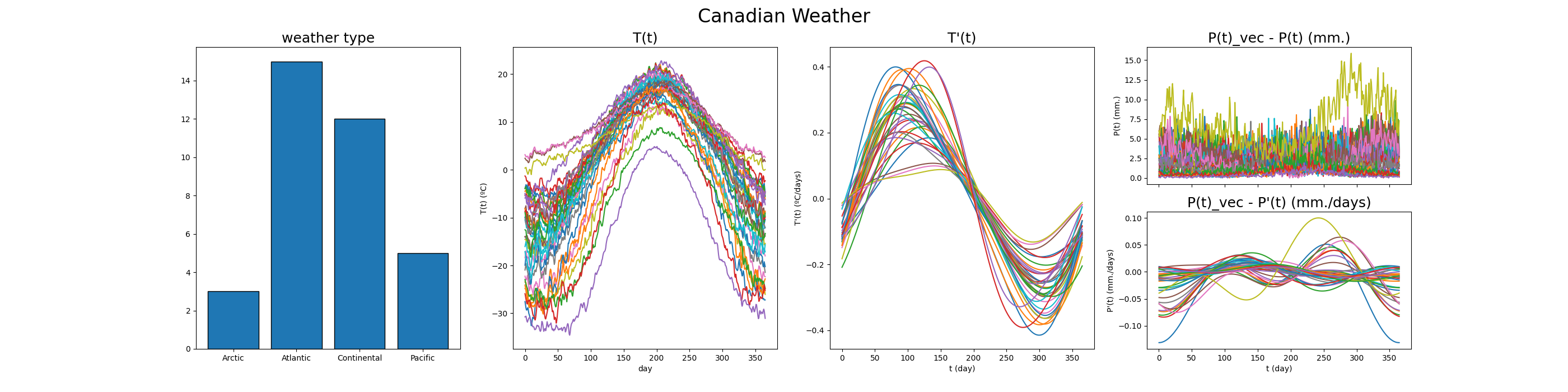
We now create a mixed data object using a pandas.DataFrame. This includes:

• a scalar variable: the climate zone (weather type),

• functional variables: the temperature \(T(t)\) and its derivative \(T'(t)\),

• and the vector-valued function combining both precipitation and its derivative: \(P_{\text{vec}}(t) = (P(t), P'(t))\).

This illustrates two valid ways to include a function and its derivative as part of the same observation.

import pandas as pd

mixed_fd = pd.DataFrame(
    {
        "weather type": y,
        "T(t)": fd_temperatures,
        "T'(t)": fd_1st_temperatures_smooth,
        "P(t)_vec": fd_vector,
    },
)

Finally, we use plot_mixed_data() to visualize the full mixed dataset. Each column is visualized with an appropriate method, helping us explore the structure in both scalar and functional components.

from skfda.exploratory.visualization.representation import plot_mixed_data

fig, axes = plt.subplots(1, 4, figsize=(28, 7))

plot_mixed_data(mixed_fd, axes=axes)
fig.suptitle("Canadian Weather", fontsize=24)
for ax in fig.axes:
    title = ax.get_title()
    if title:  # only update if there's a title
        ax.set_title(title, fontsize=18)

plt.show()