make_sde_trajectories

skfda.datasets.make_sde_trajectories(*, initial_condition, drift=None, diffusion=None, diffusion_derivative=None, n_L0_discretization_points=None, method='euler-maruyama', n_grid_points=100, n_samples=None, start=0, stop=1.0, random_state=None)

Numerical integration of an Itô SDE.

An SDE can be expressed with the following formula

\[d\mathbf{X}(t) = \mathbf{F}(t, \mathbf{X}(t))dt + \mathbf{G}(t, \mathbf{X}(t))d\mathbf{W}(t).\]

In this equation, \(\mathbf{X} = (X^{(1)}, X^{(2)}, ... , X^{(n)}) \in \mathbb{R}^q\) is a vector that represents the state of the stochastic process. The function \(\mathbf{F}(t, \mathbf{X}) = (F^{(1)}(t, \mathbf{X}), ..., F^{(q)}(t, \mathbf{X}))\) is called drift and refers to the deterministic component of the equation. The function \(\mathbf{G} (t, \mathbf{X}) = (G^{i, j}(t, \mathbf{X}))_{i=1, j=1} ^{q, m}\) is denoted as the diffusion term and refers to the stochastic component of the evolution. \(\mathbf{W}(t)\) refers to a Wiener process (Standard Brownian motion) of dimension \(m\). Finally, \(q\) refers to the dimension of the variable \(\mathbf{X}\) (dimension of the codomain) and \(m\) to the dimension of the noise.

Two methods are implemented: Euler_Maruyama’s method and Milstein’s method.

Euler-Maruyama’s method computes the approximated solution using the Markov chain

\[X_{n + 1}^{(i)} = X_n^{(i)} + F^{(i)}(t_n, \mathbf{X}_n)\Delta t_n + \sum_{j=1}^m G^{i,j}(t_n, \mathbf{X}_n)\sqrt{\Delta t_n}\Delta Z_n^j,\]

where \(X_n^{(i)}\) is the approximated value of \(X^{(i)}(t_n)\) and the \(\mathbf{Z}_m\) are independent, identically distributed \(m\)-dimensional standard normal random variables.

Milstein’s method computes the approximated solution using the Markov chain

\[X^{(i)}_{n + 1} = X_n^{(i)} + F^{(i)}(X_i, t_i)\Delta t_i + \sum_{j=1}^m G^{i,j}(t_n, X_n)\sqrt{\Delta t_n}Z_n^j + \sum_{j_1, j_2 = 1}^m L^{j_1} G^{i, j_2} (t_n, X_n) I_{(j_1, j_2)} [t_n, t_{n+1}],\]

where \(X_n^{(i)}\) is the approximated value of \(X^{(i)}(t_n)\) and the \(\mathbf{Z}_m\) are independent, identically distributed \(m\)-dimensional standard normal random variables. \(L^j\) stands for the operator

\[L^j = \sum_{k=1}^q G^{k, j}(t_n, X_n)\frac{\partial}{\partial x^k}\]

and \(I_{(j_1, j_2)} [t_n, t_{n+1}]\) is the double stochastic integral

\[I_{(j_1, j_2)} [t_n, t_{n+1}] = \int_{t_n}^{t_{n+1}} \int_{t}^{t_{n+1}} dW_s^{j_1} dW_t^{j_2}.\]

In order to compute \(I_{(j_1, j_2)} [t_n, t_{n+1}]\), we use Milstein L=0 method, described by Banerjee [1]. This method approximates the value of the double Itô integral by simulating solutions of another SDE. The number of discretization points used to simulate the SDE which approximates the double Itô integral is given by the parameter n_L0_discretization_points.

For unidimensional processes the value of the double Itô integral is closed so it is not necessary to include the n_L0_discretization_points parameter. However, if the process is multidimensional it is mandatory include it.

Parameters:

• initial_condition (ArrayLike | InitialValueGenerator) – Initial condition of the SDE. It can have one of three formats: An starting initial value from which to calculate n_samples trajectories. An array of initial values. For each starting point a trajectory will be calculated. A function that generates random numbers or vectors. It should have two parameters called size and random_state and it should return an array.

• drift (SDETerm | ArrayLike | None) – Drift term (\(F(t,\mathbf{X})\) in the equation).

• diffusion (SDETerm | ArrayLike | None) – Diffusion term (\(G(t,\mathbf{X})\) in the equation). The diffusion term should depend on the variable \(\mathbf{X}\).

• diffusion_derivative (SDETerm | None) – Derivate of the diffusion term (\(G_\mathbf{X}(t, \mathbf{X})\)). Only needed for Milstein’s method. The return of this function should have one extra dimension than the diffusion term, to account for the derivatives for each of the coordinates.

• n_L0_discretization_points (int | None) – number of discretization points to approximate the double Itô integral \(I_{(j_1,j_2)}\). Only needed in Milstein’s method. Only use when the process is multidimensional.

• method (Literal['euler-maruyama', 'milstein']) – Integration SDE method used. It can be either euler-maruyama or milstein.

• n_grid_points (int) – The total number of points of evaluation.

• n_samples (int | None) – Number of trajectories integrated.

• start (float) – Starting time of the trajectories.

• stop (float) – Ending time of the trajectories.

• random_state (RandomStateLike) – Random state.

Returns:

FDataGrid object comprising all the trajectories.

Return type:

FDataGrid

Examples

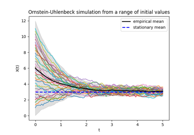
Example of the use of Euler-Maruyama’s method for an Ornstein-Uhlenbeck process that has the equation:

>>> from scipy.stats import norm
>>> A = 1
>>> mu = 3
>>> B = 0.5
>>> def ou_drift(t: float, x: np.ndarray) -> np.ndarray:
...     return -A * (x - mu)
>>> initial_condition = norm().rvs
>>>
>>> trajectories = make_sde_trajectories(
...     initial_condition=initial_condition,
...     n_samples=10,
...     drift=ou_drift,
...     diffusion=B,
... )

Example of the use of Milstein’s method for a 1-d Geometric Brownian motion that has the equation:

>>> sigma = 1
>>> mu = 2
>>> def gbm_drift(t: float, x: np.ndarray) -> np.ndarray:
...     return mu * x
>>> def gbm_diffusion(t: float, x: np.ndarray) -> np.ndarray:
...     return sigma * x
>>> def gbm_diff_derivative(t: float, x: np.ndarray) -> np.ndarray:
...     return sigma * np.ones_like(x)[: :, np.newaxis]
>>> X_0 = 1
>>> n_L0_discretization_points = 5,
>>>
>>> trajectories = make_sde_trajectories(
...     initial_condition=X_0,
...     drift=gbm_drift,
...     diffusion=gbm_diffusion,
...     diffusion_derivative=gbm_diff_derivative,
...     n_L0_discretization_points=n_L0_discretization_points,
...     method="milstein",
...     n_samples=10,
... )

References

[1]

Paromita Banerjee. Numerical Methods for Stochastic Differential Equations and Postintervention in Structural Equation Models. PhD thesis, Case Western Reserve University, USA, 2020.

Examples using skfda.datasets.make_sde_trajectories

SDE simulation: Langevin dynamics

SDE simulation: Langevin dynamics

SDE simulation: creating synthetic datasets using SDEs

SDE simulation: creating synthetic datasets using SDEs