Note
Go to the end to download the full example code. or to run this example in your browser via Binder
Mixed effects model for irregular data: robustness of the conversion#
This example converts irregular data to a basis representation using a mixed effects model and checks the robustness of the method by fitting the model with decreasing number of measurement points per curve.
# Author: Pablo Cuesta Sierra
# License: MIT

# sphinx_gallery_thumbnail_number = -1
For this example, we are going to check the robustness of the mixed effects method for converting irregular data to basis representation by removing some measurement points from the test and train sets and comparing the resulting conversions.
The temperatures from the Canadian weather dataset are used to generate the irregular data. We use a Fourier basis due to the periodic nature of the data.
import matplotlib.pyplot as plt

from skfda.datasets import fetch_weather
from skfda.representation.basis import FourierBasis

fd_temperatures = fetch_weather().data.coordinates[0]
basis = FourierBasis(n_basis=5, domain_range=fd_temperatures.domain_range)
We plot the original data and the basis functions.
fig, axes = plt.subplots(1, 2, figsize=(10, 4))

ax = axes[0]
fd_temperatures.plot(axes=ax)
ylim = ax.get_ylim()
xlabel = ax.get_xlabel()
ax.set_title(fd_temperatures.dataset_name)

ax = axes[1]
basis.plot(axes=ax)
ax.set_xlabel(xlabel)
ax.set_title("Basis functions")

fig.suptitle("")
plt.show()

We split the data into train and test sets:
import numpy as np
from sklearn.model_selection import train_test_split

from skfda import FDataIrregular

random_state = np.random.RandomState(seed=13627798)
train_original, test_original = train_test_split(
    fd_temperatures,
    test_size=0.3,
    random_state=random_state,
)
test_original_irregular = FDataIrregular.from_fdatagrid(test_original)
Then, we create datasets with decreasing number of measurement points per curve, by removing measurement points from the previous dataset iteratively.
from skfda.datasets import irregular_sample

n_points_list = [365, 40, 10, 7, 5, 4, 3]
train_irregular_datasets = []
test_irregular_datasets = []
current_train = train_original
current_test = test_original
for n_points in n_points_list:
    current_train = irregular_sample(
        current_train,
        n_points_per_curve=n_points,
        random_state=random_state,
    )
    current_test = irregular_sample(
        current_test,
        n_points_per_curve=n_points,
        random_state=random_state,
    )
    train_irregular_datasets.append(current_train)
    test_irregular_datasets.append(current_test)
We now define with measures will we track for score or error.
from skfda.misc.scoring import mean_squared_error, r2_score

score_functions = {
    "R^2": r2_score,
    "MSE": mean_squared_error,
}
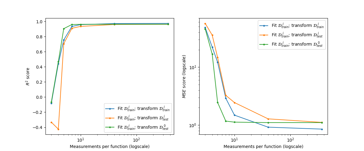
We convert the irregular data to basis representation and compute the scores. To do so, we fit the converter once per train set. After fitting the the converter with a train set that has \(k\) points per curve, we use it to transform that train set, the test set with \(k\) points per curve and the original test set with 365 points per curve.
import pandas as pd

from skfda.representation.conversion import EMMixedEffectsConverter

converter = EMMixedEffectsConverter(basis)


# Store the converted data
converted_data = {
    "Train-sparse": [],
    "Test-sparse": [],
    "Test-original": [],
}
for train_irregular, test_irregular in zip(
    train_irregular_datasets,
    test_irregular_datasets,
    strict=True,
):
    converter = converter.fit(train_irregular)

    converted_data["Train-sparse"].append(
        converter.transform(train_irregular),
    )
    converted_data["Test-sparse"].append(
        converter.transform(test_irregular),
    )
    converted_data["Test-original"].append(
        converter.transform(test_original_irregular),
    )

# Calculate and store the scores
scores = {
    score_name: pd.DataFrame(
        {
            data_name: [
                score_fun(
                    test_original if "Test" in data_name else train_original,
                    transformed.to_grid(test_original.grid_points),
                )
                for transformed in converted_data[data_name]
            ]
            for data_name in converted_data
        },
        index=pd.Index(n_points_list, name="Points per curve"),
    )
    for score_name, score_fun in score_functions.items()
}
Finally, we have the scores for the train and test sets with decreasing number of measurement points per curve.
The \(R^2\) scores are as follows (higher is better):
scores["R^2"]
The MSE errors are as follows (lower is better):
scores["MSE"]
Plot the scores.
label_train = r"$\mathcal{D}_{train}^{\ j}$"
label_test = r"$\mathcal{D}_{test}^{\ j}$"
label_test_orig = r"$\mathcal{D}_{test}^{\ 0}$"

fig, axes = plt.subplots(1, 2, figsize=(12, 5))
for i, (score_name, values) in enumerate(scores.items()):
    ax = axes[i]
    ax.plot(
        values.index,
        values["Train-sparse"],
        label=f"Fit {label_train}; transform {label_train}",
        marker=".",
    )
    ax.plot(
        values.index,
        values["Test-sparse"],
        label=f"Fit {label_train}; transform {label_test}",
        marker=".",
    )
    ax.plot(
        values.index,
        values["Test-original"],
        label=f"Fit {label_train}; transform {label_test_orig}",
        marker=".",
    )
    if score_name == "MSE":
        ax.set_yscale("log")
        ax.set_ylabel(f"${score_name}$ score (logscale)")
    else:
        ax.set_ylabel(f"${score_name}$ score")

    ax.set_xscale("log")
    ax.set_xlabel(r"Measurements per function (logscale)")
    ax.legend()

plt.show()
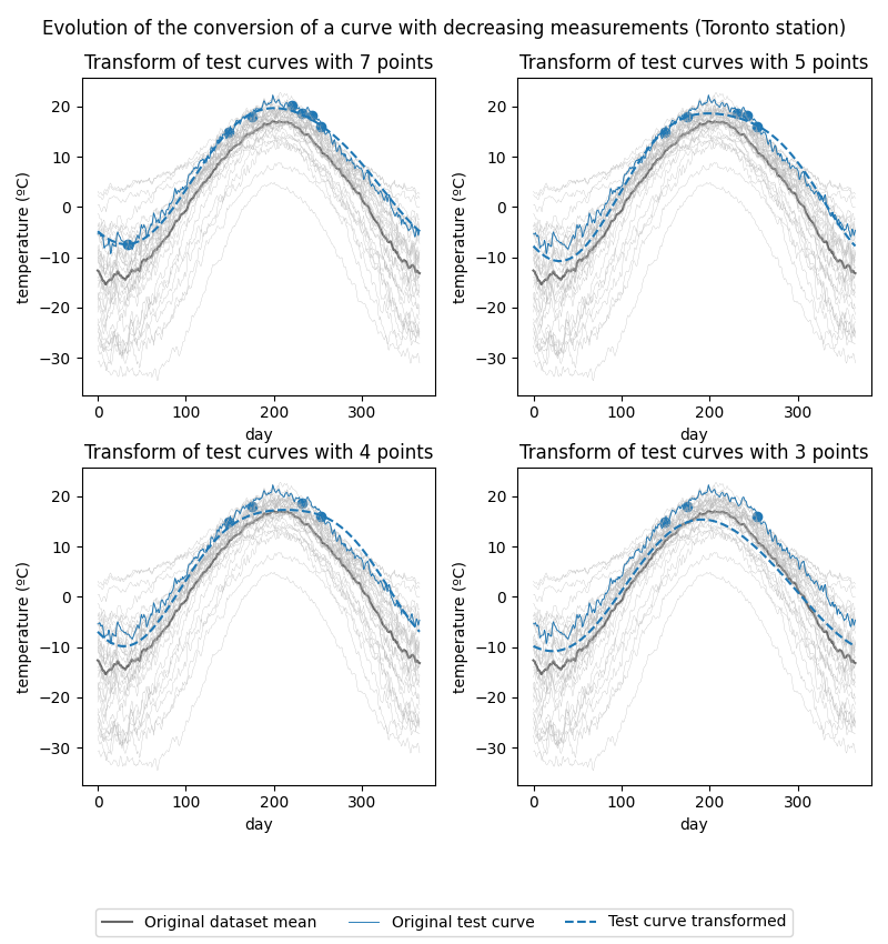
Show the original curves along with the converted test curves for the conversions with 7, 5, 4 and 3 points per curve.
def plot_conversion_evolution(index: int) -> None:
    """Plot evolution of the conversion for a particular curve."""
    fig, axes = plt.subplots(2, 2, figsize=(8, 8.5))
    start_index = 3
    for i, n_points_per_curve in enumerate(n_points_list[start_index:]):

        ax = axes.flat[i]

        test_irregular_datasets[i + start_index][index].scatter(
            axes=ax,
            color="C0",
        )
        fd_temperatures.mean().plot(
            axes=ax,
            color=[0.4] * 3,
            label="Original dataset mean",
        )
        fd_temperatures.plot(
            axes=ax,
            color=[0.7] * 3,
            linewidth=0.2,
        )
        test_original[index].plot(
            axes=ax,
            color="C0",
            linewidth=0.65,
            label="Original test curve",
        )
        converted_data["Test-sparse"][i + start_index][index].plot(
            axes=ax,
            color="C0",
            linestyle="--",
            label="Test curve transformed",
        )
        ax.set_title(
            f"Transform of test curves with {n_points_per_curve} points",
        )
        ax.set_ylim(ylim)

    fig.suptitle(
        "Evolution of the conversion of a curve with decreasing measurements "
        f"({test_original.sample_names[index]} station)",
    )

    # Add common legend at the bottom:
    handles, labels = ax.get_legend_handles_labels()
    fig.tight_layout(h_pad=0, rect=(0, 0.1, 1, 1))
    fig.legend(
        handles=handles,
        loc="lower center",
        ncols=3,
    )

    plt.show()
Toronto station’s temperature curve conversion evolution:
plot_conversion_evolution(index=7)
Iqaluit station’s temperature curve conversion evolution:
plot_conversion_evolution(index=8)
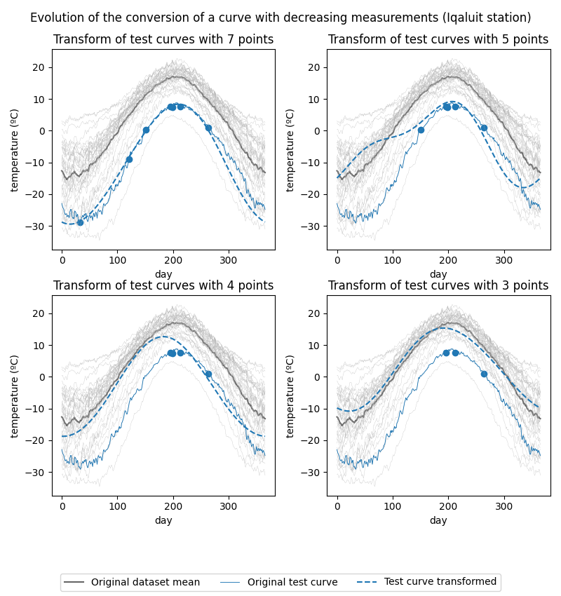
As can be seen in the figures, the fewer the measurements, the closer the converted curve is to the mean of the original dataset. This leads us to believe that when the amount of measurements is too low, the mixed-effects model is able to capture the general trend of the data, but it is not able to properly capture the individual variation of each curve.
Total running time of the script: (0 minutes 19.843 seconds)