Exploring data

Explores the Tecator data set by plotting the functional data and calculating means and derivatives.

# Author: Miguel Carbajo Berrocal
# License: MIT

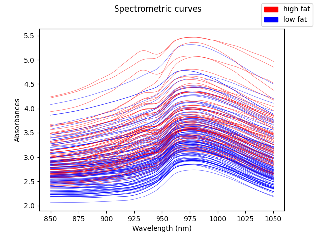
In this example we are going to explore the functional properties of the Tecator dataset. This dataset measures the infrared absorbance spectrum of meat samples. The objective is to predict the fat, water, and protein content of the samples.

In this example we only want to discriminate between meat with less than 20% of fat, and meat with a higher fat content.

from skfda.datasets import fetch_tecator

X, y = fetch_tecator(return_X_y=True, as_frame=True)
fd = X.iloc[:, 0].array
fat = y["fat"].to_numpy()

We will now plot in red samples containing less than 20% of fat and in blue the rest.

import matplotlib.pyplot as plt
import numpy as np

fat_threshold_percent = 20
low_fat = fat < fat_threshold_percent
labels = np.full(fd.n_samples, "high fat")
labels[low_fat] = "low fat"
colors = {
    "high fat": "red",
    "low fat": "blue",
}

fd.plot(
    group=labels,
    group_colors=colors,
    linewidth=0.5,
    alpha=0.7,
    legend=True,
)
plt.show()

The means of each group are the following ones.

from skfda.exploratory.stats import mean

mean_low = mean(fd[low_fat])
mean_high = mean(fd[~low_fat])

means = mean_high.concatenate(mean_low)

means.dataset_name = f"{fd.dataset_name} - means"
means.plot(
    group=["high fat", "low fat"],
    group_colors=colors,
    linewidth=0.5,
    legend=True,
)
plt.show()

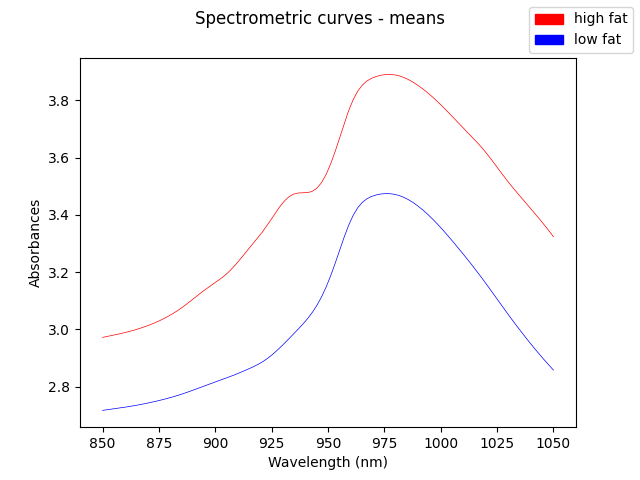
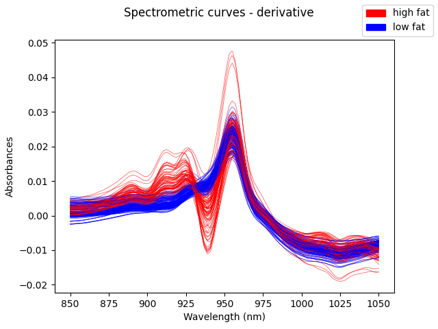
In this dataset, the vertical shift in the original trajectories is not very significative for predicting the fat content. However, the shape of the curve is very relevant. We can observe that looking at the first and second derivatives.

The first derivative is shown below:

fdd = fd.derivative()
fdd.dataset_name = f"{fd.dataset_name} - derivative"
fdd.plot(
    group=labels,
    group_colors=colors,
    linewidth=0.5,
    alpha=0.7,
    legend=True,
)
plt.show()

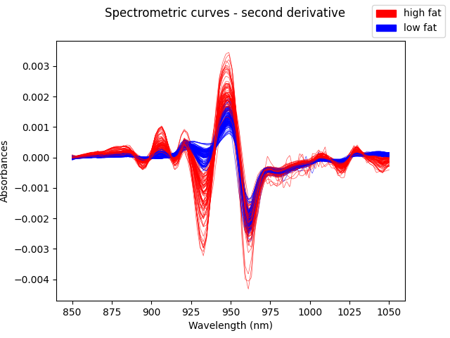
We now show the second derivative:

fdd = fd.derivative(order=2)
fdd.dataset_name = f"{fd.dataset_name} - second derivative"
fdd.plot(
    group=labels,
    group_colors=colors,
    linewidth=0.5,
    alpha=0.7,
    legend=True,
)
plt.show()