Functional Principal Component Analysis Regression.

This example explores the use of the functional principal component analysis (FPCA) in regression problems.

# Author: David del Val
# License: MIT

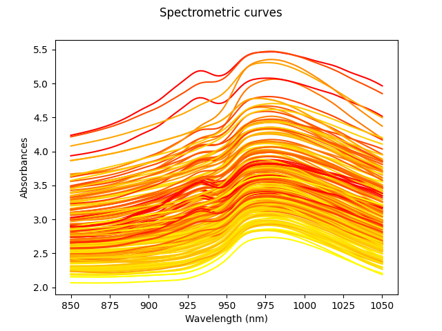
In this example, we will demonstrate the use of the FPCA regression method using the tecator dataset. This data set contains 215 samples. Each of those samples is comprised of a spectrum of absorbances and the contents of water, fat and protein.

from skfda.datasets import fetch_tecator

X_df, y_df = fetch_tecator(return_X_y=True, as_frame=True)
X = X_df.iloc[:, 0].array
y = y_df["fat"].to_numpy()

Our goal will be to estimate the fat percentage from the spectrum. However, in order to better understand the data, we will first plot all the spectra curves. The color of these curves depends on the amount of fat, from least (yellow) to highest (red).

import matplotlib.pyplot as plt

X.plot(gradient_criteria=y, legend=True)
plt.show()

In order to evaluate the performance of the model, we will split the data into train and test sets. The former will contain 80% of the samples, while the latter will contain the remaining 20%.

from sklearn.model_selection import train_test_split

X_train, X_test, y_train, y_test = train_test_split(
    X,
    y,
    test_size=0.2,
    random_state=1,
)

Since the FPCA regression provides good results with a small number of components, we will start by using only 5 components. After training the model, we can check its performance on the test set.

from skfda.ml.regression import FPCARegression

reg = FPCARegression(n_components=5)
reg.fit(X_train, y_train)
test_score = reg.score(X_test, y_test)
print(f"Score with 5 components: {test_score:.4f}")

Score with 5 components: 0.9062

We have obtained a pretty good result considering that the model has only used 5 components. That is to say, the dimensionality of the problem has been reduced from 100 (each spectrum has 100 points) to 5.

However, we can improve the performance of the model by using more components. To do so, we will use cross validation to find the best number of components. We will test with values from 1 to 100.

from sklearn.model_selection import GridSearchCV

param_grid = {"n_components": range(1, 100, 1)}
reg = FPCARegression()

# Perform grid search with cross-validation
gscv = GridSearchCV(reg, param_grid, cv=5)
gscv.fit(X_train, y_train)


print("Best params:", gscv.best_params_)
print(f"Best cross-validation score: {gscv.best_score_:.4f}")

Best params: {'n_components': 28}
Best cross-validation score: 0.9652

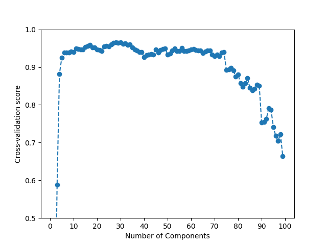
The best performance for the train set is obtained using 30 components. This still provides a good reduction in dimensionality. However, it is important to note that the performance of the model scales very slowly with the number of components.

This phenomenon can be seen in the following plot, and confirms that FPCA already provides a good approximation of the data with a small number of components.

fig = plt.figure()
ax = fig.add_subplot(1, 1, 1)
ax.plot(
    param_grid["n_components"],
    gscv.cv_results_["mean_test_score"],
    linestyle="dashed",
    marker="o",
)
ax.set_xticks(range(0, 110, 10))
ax.set_xlabel("Number of Components")
ax.set_ylabel("Cross-validation score")
ax.set_ylim((0.5, 1))
fig.show()

To conclude, we can calculate the score of the model on the test set after it has been trained on the whole train set.

Moreover, we can check that the score barely changes when we use a somewhat smaller number of components.

reg = FPCARegression(n_components=30)
reg.fit(X_train, y_train)
test_score = reg.score(X_test, y_test)
print(f"Score with 30 components: {test_score:.4f}")

reg = FPCARegression(n_components=15)
reg.fit(X_train, y_train)
test_score = reg.score(X_test, y_test)
print(f"Score with 15 components: {test_score:.4f}")

Score with 30 components: 0.9667
Score with 15 components: 0.9584