Voice signals: smoothing, registration, and classification

Shows the use of functional preprocessing tools such as smoothing and registration, and functional classification methods.

# License: MIT

# sphinx_gallery_thumbnail_number = 3

This example uses the Phoneme dataset[1] containing the frequency curves of some common phonemes as pronounced by different people. We illustrate with this data the preprocessing and classification techniques available in scikit-fda.

This is one of the examples presented in the ICTAI conference[2].

We will first load the (binary) Phoneme dataset and plot the first 20 functions. We restrict the data to the first 150 variables, as done in Ferraty and Vieu (chapter 7)[3], because most of the useful information is in the lower frequencies.

import matplotlib.pyplot as plt
import numpy as np

from skfda.datasets import fetch_phoneme

X, y = fetch_phoneme(return_X_y=True)

X = X[(y == 0) | (y == 1)]
y = y[(y == 0) | (y == 1)]

n_points = 150

new_points = X.grid_points[0][:n_points]
new_data = X.data_matrix[:, :n_points]

X = X.copy(
    grid_points=new_points,
    data_matrix=new_data,
    domain_range=(float(np.min(new_points)), float(np.max(new_points))),
)

n_plot = 20
X[:n_plot].plot(group=y)
plt.show()

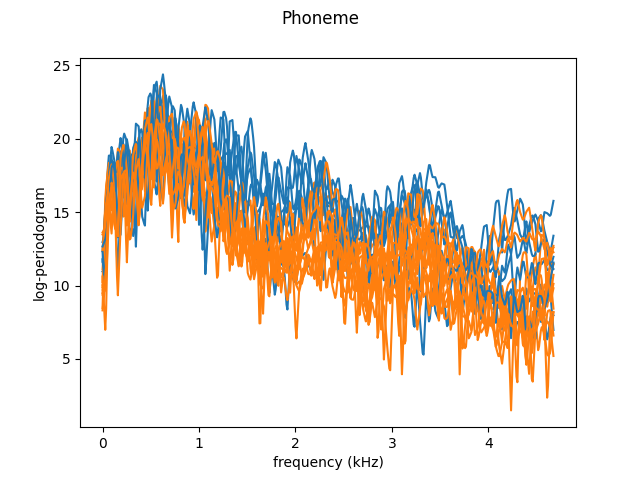
As we just saw, the curves are very noisy. We can leverage the continuity of the trajectories by smoothing, using a Nadaraya-Watson estimator. We then plot the data again, as well as the class means.

from skfda.misc.hat_matrix import NadarayaWatsonHatMatrix
from skfda.misc.kernels import normal
from skfda.preprocessing.smoothing import KernelSmoother

smoother = KernelSmoother(
    NadarayaWatsonHatMatrix(
        bandwidth=0.1,
        kernel=normal,
    ),
)
X_smooth = smoother.fit_transform(X)

fig = X_smooth[:n_plot].plot(group=y)

X_smooth_aa = X_smooth[:n_plot][y[:n_plot] == 0]
X_smooth_ao = X_smooth[:n_plot][y[:n_plot] == 1]

X_smooth_aa.mean().plot(fig=fig, color="blue", linewidth=3)
X_smooth_ao.mean().plot(fig=fig, color="red", linewidth=3)
plt.show()

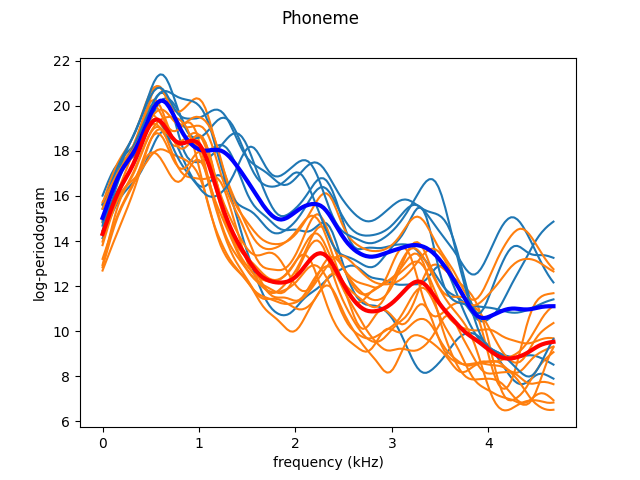
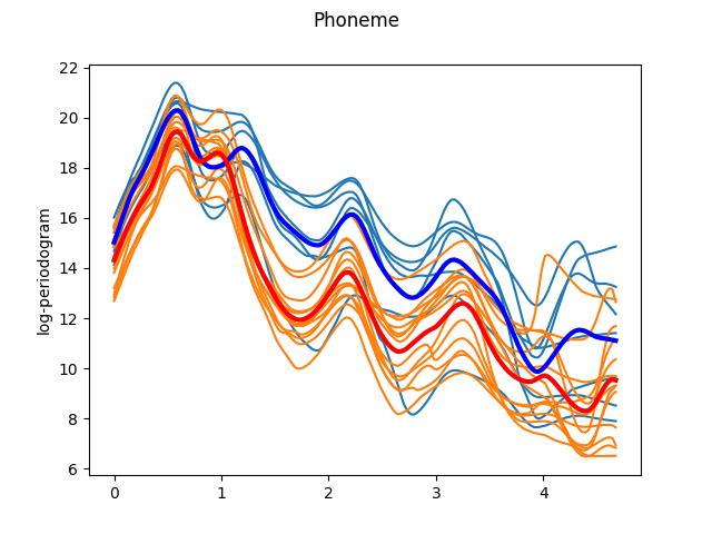
The smoothed curves are easier to interpret. Now, it is possible to appreciate the characteristic landmarks of each class, such as maxima or minima. However, not all these landmarks appear at the same frequency for each trajectory. One way to solve it is by registering (aligning) the data. We use Fisher-Rao elastic registration, a state-of-the-art registration method to illustrate the effect of registration. Although this registration method achieves very good results, it attempts to align all the curves to a common template. Thus, in order to clearly view the specific landmarks of each class we have to register the data per class. This also means that if the we cannot use this method for a classification task if the landmarks of each class are very different, as it is not able to do per-class registration with unlabeled data. As Fisher-Rao elastic registration is very slow, we only register the plotted curves as an approximation.

from skfda.preprocessing.registration import FisherRaoElasticRegistration

reg = FisherRaoElasticRegistration(
    penalty=0.01,
)

X_reg_aa = reg.fit_transform(X_smooth[:n_plot][y[:n_plot] == 0])
fig = X_reg_aa.plot(color="C0")

X_reg_ao = reg.fit_transform(X_smooth[:n_plot][y[:n_plot] == 1])
X_reg_ao.plot(fig=fig, color="C1")

X_reg_aa.mean().plot(fig=fig, color="blue", linewidth=3)
X_reg_ao.mean().plot(fig=fig, color="red", linewidth=3)
plt.show()

We now split the smoothed data in train and test datasets. Note that there is no data leakage because no parameters are fitted in the smoothing step, but normally you would want to do all preprocessing in a pipeline to guarantee that.

from sklearn.model_selection import train_test_split

X_train, X_test, y_train, y_test = train_test_split(
    X_smooth,
    y,
    test_size=0.25,
    random_state=0,
    stratify=y,
)

We use a k-nn classifier with a functional analog to the Mahalanobis distance and a fixed number of neighbors.

from sklearn.metrics import accuracy_score

from skfda.misc.metrics import MahalanobisDistance
from skfda.ml.classification import KNeighborsClassifier

n_neighbors = int(np.sqrt(X_smooth.n_samples))
n_neighbors += n_neighbors % 2 - 1  # Round to an odd integer

classifier = KNeighborsClassifier(
    n_neighbors=n_neighbors,
    metric=MahalanobisDistance(
        alpha=0.001,
    ),
)

classifier.fit(X_train, y_train)
y_pred = classifier.predict(X_test)
score = accuracy_score(y_test, y_pred)
print(score)

0.8046511627906977

If we wanted to optimize hyperparameters, we can use scikit-learn tools.

from sklearn.model_selection import GridSearchCV
from sklearn.pipeline import Pipeline

pipeline = Pipeline([
    ("smoother", smoother),
    ("classifier", classifier),
])

grid_search = GridSearchCV(
    pipeline,
    param_grid={
        "smoother__kernel_estimator__bandwidth": [1, 1e-1, 1e-2, 1e-3],
        "classifier__n_neighbors": range(3, n_neighbors, 2),
        "classifier__metric__alpha": [1, 1e-1, 1e-2, 1e-3, 1e-4],
    },
)

# The grid search is too slow for a example. Uncomment it if you want, but it
# will take a while.

# grid_search.fit(X_train, y_train)
# y_pred = grid_search.predict(X_test)
# score = accuracy_score(y_test, y_pred)
# print(score)

The optimal parameters obtained are smoother__kernel_estimator__bandwidth = 0.01, classifier__n_neighbors = 37 and classifier__metric__alpha = 0.001. We now train a new classifier with these parameters.

optimal_smoother = KernelSmoother(
    NadarayaWatsonHatMatrix(
        bandwidth=0.01,
        kernel=normal,
    ),
)

optimal_classifier = KNeighborsClassifier(
    n_neighbors=37,
    metric=MahalanobisDistance(
        alpha=0.001,
    ),
)

optimal_pipeline = Pipeline([
    ("smoother", optimal_smoother),
    ("classifier", optimal_classifier),
])

optimal_pipeline.fit(X_train, y_train)
y_pred = optimal_pipeline.predict(X_test)
score = accuracy_score(y_test, y_pred)
print(f"Accuracy of the optimized pipeline: {score:.4f}")

Accuracy of the optimized pipeline: 0.8023

References

[1]

Trevor Hastie, Andreas Buja, and Robert Tibshirani. Penalized discriminant analysis. The Annals of Statistics, 23(1):73–102, February 1995. URL: https://projecteuclid.org/euclid.aos/1176324456 (visited on 2018-12-09), doi:10.1214/aos/1176324456.

[2]

Carlos Ramos-Carreño, José Luis Torrecilla, Yujian Hong, and Alberto Suárez. scikit-fda: Computational tools for machine learning with functional data. In 2022 IEEE 34th International Conference on Tools with Artificial Intelligence (ICTAI), 213–218. October 2022. doi:10.1109/ICTAI56018.2022.00038.

[3]

Frédéric Ferraty and Philippe Vieu. Nonparametric Functional Data Analysis: Theory and Practice. Springer Series in Statistics. Springer-Verlag, New York, 2006. ISBN 978-0-387-30369-7. URL: https://www.springer.com/gp/book/9780387303697 (visited on 2019-09-10).