Functional Diffusion Maps

In this example, the use of the functional diffusion map (FDM) technique is shown over different datasets. Firstly, an example of basic use of the technique is provided. Later, two examples of parameter tuning are presented, for embedding spaces of diferent dimensions. Finally, an application of the method for a real, non-synthetic, dataset is provided.

# Author: Eduardo Terrés Caballero
# License: MIT

Some examples shown here are further explained in the article Barroso et al.[1].

Moons dataset example

Firstly, a basic example of execution is presented using a functional version of the moons dataset, a dataset consisting of two dimentional coordinates representing the position of two different moons.

import matplotlib.pyplot as plt
import numpy as np
from matplotlib.colors import ListedColormap
from sklearn import datasets

seed = 612245103
random_state = np.random.RandomState(seed)

n_samples, n_grid_pts = 100, 50
data_moons, y = datasets.make_moons(
    n_samples=n_samples,
    noise=0,
    random_state=random_state,
)

colors = ["blue", "orange"]
cmap = ListedColormap(colors)
fig, ax = plt.subplots()
ax.scatter(data_moons[:, 0], data_moons[:, 1], c=y, cmap=cmap)
ax.set_title("Moons data")
plt.show()

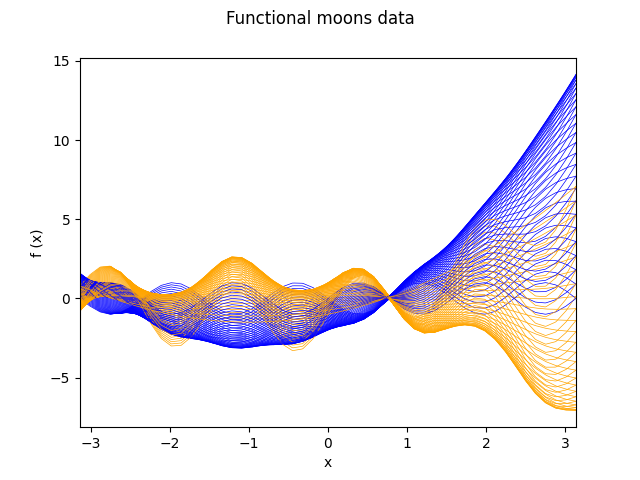
Using a two elements basis, the functional observation corresponding to a multivariate observation is obtained by treating the coordinates as coefficients that multiply the elements of the basis. In other words, the multivariate vectors are interpreted as elements of the basis. Below is the code to generate the synthetic moons functional data.

from skfda.representation import FDataGrid

grid = np.linspace(-np.pi, np.pi, n_grid_pts)
basis = np.array([np.sin(4 * grid), grid ** 2 + 2 * grid - 2])
fd_moons = FDataGrid(
    data_matrix=data_moons @ basis,
    grid_points=grid,
    dataset_name="Functional moons data",
    argument_names=("x",),
    coordinate_names=("f (x)",),
)
fig = fd_moons.plot(linewidth=0.5, group=y, group_colors=colors)
fig.axes[0].set_xlim((-np.pi, np.pi))
plt.show()

Once the functional data is available, it simply remains to choose the value of the parameters of the model.

The FDM technique involves the use of a kernel operator, that acts as a measure of similarity for the data. In this case we will be using the Gaussian kernel, with a length scale parameter of 0.25.

from skfda.misc.covariances import Gaussian
from skfda.preprocessing.dim_reduction import DiffusionMap

fdm = DiffusionMap(
    n_components=2,
    kernel=Gaussian(length_scale=0.25),
    alpha=0,
    n_steps=1,
)
embedding = fdm.fit_transform(fd_moons)

fig, ax = plt.subplots()
ax.scatter(embedding[:, 0], embedding[:, 1], c=y, cmap=cmap)
ax.set_title("Diffusion coordinates for the functional moons data")
plt.show()

As we can see, the functional diffusion map has correctly interpreted the topological nature of the data, by successfully separating the coordinates associated to both moons.

Spirals dataset example

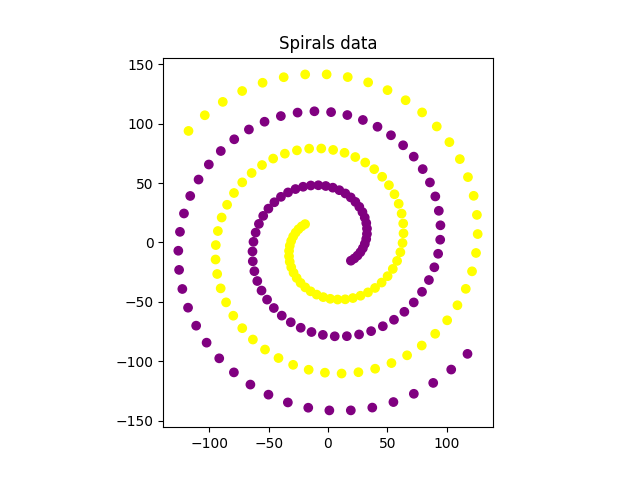
Next is an example of parameter tuning in the form of a grid search for a set of given values for the length_scale kernel parameter and the alpha parameter of the FDM method. We have two spirals, which are initially entangled and thus indistinguishable to the machine.

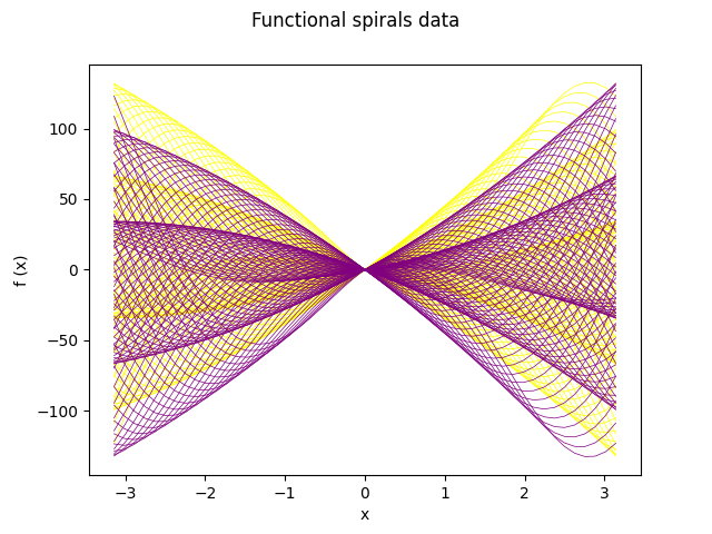
Below is the code for the generation of the spiral data and its functional equivalent, following a similar dynamic as in the moons dataset.

n_samples, n_grid_pts = 100, 50
t = (np.pi / 4 + np.linspace(0, 4, n_samples)) * np.pi
dx, dy = 10 * t * np.cos(t), 10 * t * np.sin(t)
y = np.array([0] * n_samples + [1] * n_samples)
data_spirals = np.column_stack((
    np.concatenate((dx, -dx)), np.concatenate((dy, -dy)),
))

colors = ["yellow", "purple"]
cmap = ListedColormap(colors)
fig, ax = plt.subplots()
ax.scatter(data_spirals[:, 0], data_spirals[:, 1], c=y, cmap=cmap)
ax.set_aspect("equal", adjustable="box")
ax.set_title("Spirals data")
plt.show()

# Define functional data object
grid = np.linspace(-np.pi, np.pi, n_grid_pts)
basis = np.array([grid * np.cos(grid) / 3, grid * np.sin(grid) / 3])
fd_spirals = FDataGrid(
    data_matrix=data_spirals @ basis,
    grid_points=grid,
    dataset_name="Functional spirals data",
    argument_names=("x",),
    coordinate_names=("f (x)",),
)
fd_spirals.plot(linewidth=0.5, group=y, group_colors=colors)
plt.show()

• 
• 

Once the functional data is ready, we will perform a grid search for the following values of the parameters, as well as plot the resulting embeddings for visual comparison.

from itertools import product

alpha_set = [0, 0.33, 0.66, 1]
length_scale_set = [2.5, 3, 4.5, 7, 10, 11, 15]
param_grid = product(alpha_set, length_scale_set)

fig, axes = plt.subplots(
    len(alpha_set), len(length_scale_set), figsize=(16, 8),
)

for (alpha, length_scale), ax in zip(param_grid, axes.ravel(), strict=True):
    fdm = DiffusionMap(
        n_components=2,
        kernel=Gaussian(length_scale=length_scale),
        alpha=alpha,
        n_steps=1,
    )
    embedding = fdm.fit_transform(fd_spirals)

    ax.scatter(embedding[:, 0], embedding[:, 1], c=y, cmap=cmap)
    ax.set_xticklabels([])
    ax.set_yticklabels([])

for ax, alpha in zip(axes[:, 0], alpha_set, strict=True):
    ax.set_ylabel(f"$\\alpha$: {alpha}", size=20, rotation=0, ha="right")

for ax, length_scale in zip(axes[0], length_scale_set, strict=True):
    ax.set_title(f"$len-sc$: {length_scale}", size=20, va="bottom")

plt.show()

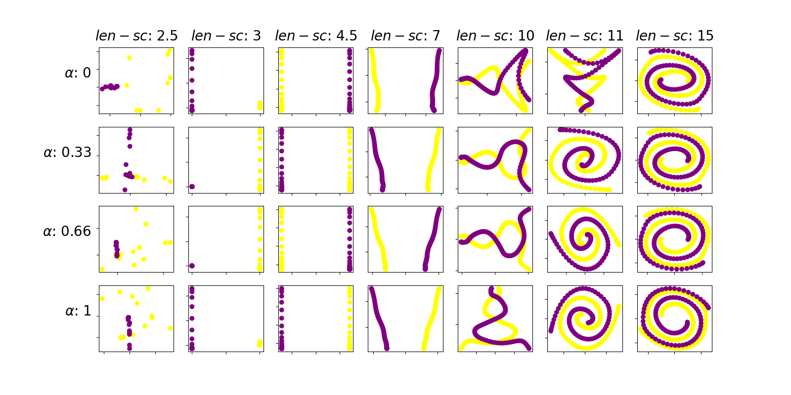
The first thing to notice is that the parameter length scale exerts a greater influence in the resulting embedding than the parameter alpha. In this sense, the figures of any given column are more similar than those of any given row. Thus, we shall set alpha equal to 0 because, by theory, it is equivalent to skipping a normalization step in the process

Moreover, we can see that the optimal choice of the length scale parameter of the kernel is 4.5 because it visually presents the more clear separation between the trajectories of both spirals. Hence, for a length scale of the kernel function of 4.5 the method is able to understand the local geometry of the spirals dataset. For a small value of the kernel parameter (for example 1) contiguous points in the same arm of the spiral are not considered close because the kernel is too narrow, resulting in apparently random diffusion coordinates. For a large value of the kernel parameter (for example 15) the kernel is wide enough so that points in contiguous spiral arms, which belong to different trajectories, are considered similar. Hence the diffusion coordinates keep these relations by mantaining both trajectories entagled. In summary, for a value of length scale of 4.5 the kernel is wide enough so that points in the same arm of a trajectory are considered similar, but its not too wide so that points in contiguous arms of the spiral are also considered similar.

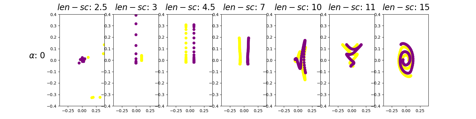
For a reliable comparison between embeddings, it is advisable to use the same scale in all axis. To ilustrate this idea, next is a re-execution for the row alpha equals 0.

alpha_set = [0]
length_scale_set = [2.5, 3, 4.5, 7, 10, 11, 15]
param_grid = product(alpha_set, length_scale_set)

fig, axes = plt.subplots(
    len(alpha_set),
    len(length_scale_set),
    figsize=(16, 4),
)

for (alpha, length_scale), ax in zip(param_grid, axes.ravel(), strict=True):
    fdm = DiffusionMap(
        n_components=2,
        kernel=Gaussian(length_scale=length_scale),
        alpha=alpha,
        n_steps=1,
    )
    embedding = fdm.fit_transform(fd_spirals)

    ax.scatter(embedding[:, 0], embedding[:, 1], c=y, cmap=cmap)
    ax.set_xlim((-0.4, 0.4))
    ax.set_ylim((-0.4, 0.4))

axes[0].set_ylabel(
    f"$\\alpha$: {alpha_set[0]}", size=20, rotation=0, ha="right",
)

for ax, length_scale in zip(axes, length_scale_set, strict=True):
    ax.set_title(f"$len-sc$: {length_scale}", size=20, va="bottom")

plt.show()

Swiss roll dataset example

So far, the above examples have been computed with a value of the n_components parameter of 2. This implies that the resulting diffusion coordinate points belong to a two-dimensional space and thus we can provide a graphical representation. The aim of this new section is to explore further possibilities regarding n_components.

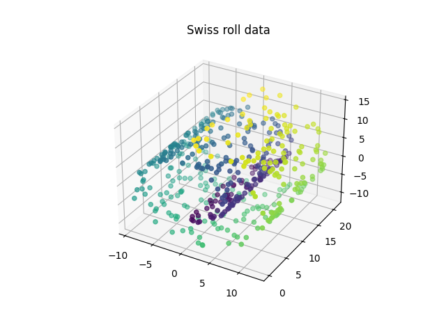
We will now apply the method to a more complex example, the Swiss roll dataset. This dataset consists of three dimensional points that lay over a topological manifold shaped like a Swiss roll.

n_samples, n_grid_pts = 500, 100
data_swiss, y = datasets.make_swiss_roll(
    n_samples=n_samples,
    noise=0,
    random_state=random_state,
)
fig = plt.figure()
axis = fig.add_subplot(111, projection="3d")
axis.set_title("Swiss roll data")
axis.scatter(data_swiss[:, 0], data_swiss[:, 1], data_swiss[:, 2], c=y)
plt.show()

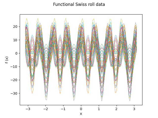
Similarly to the previous examples, the functional data object is defined. In this case a three element base will be used, since the multivariate data points belong to a three-dimensional space. For clarity purposes, only the first fifty functional observations are plotted.

grid = np.linspace(-np.pi, np.pi, n_grid_pts)
basis = np.array([np.sin(4 * grid), np.cos(8 * grid), np.sin(12 * grid)])
data_matrix = np.array(data_swiss) @ basis
fd_swiss = FDataGrid(
    data_matrix=data_matrix,
    grid_points=grid,
    dataset_name="Functional Swiss roll data",
    argument_names=("x",),
    coordinate_names=("f (x)",),
)
fd_swiss[:50].plot(linewidth=0.5, group=y[:50])
plt.show()

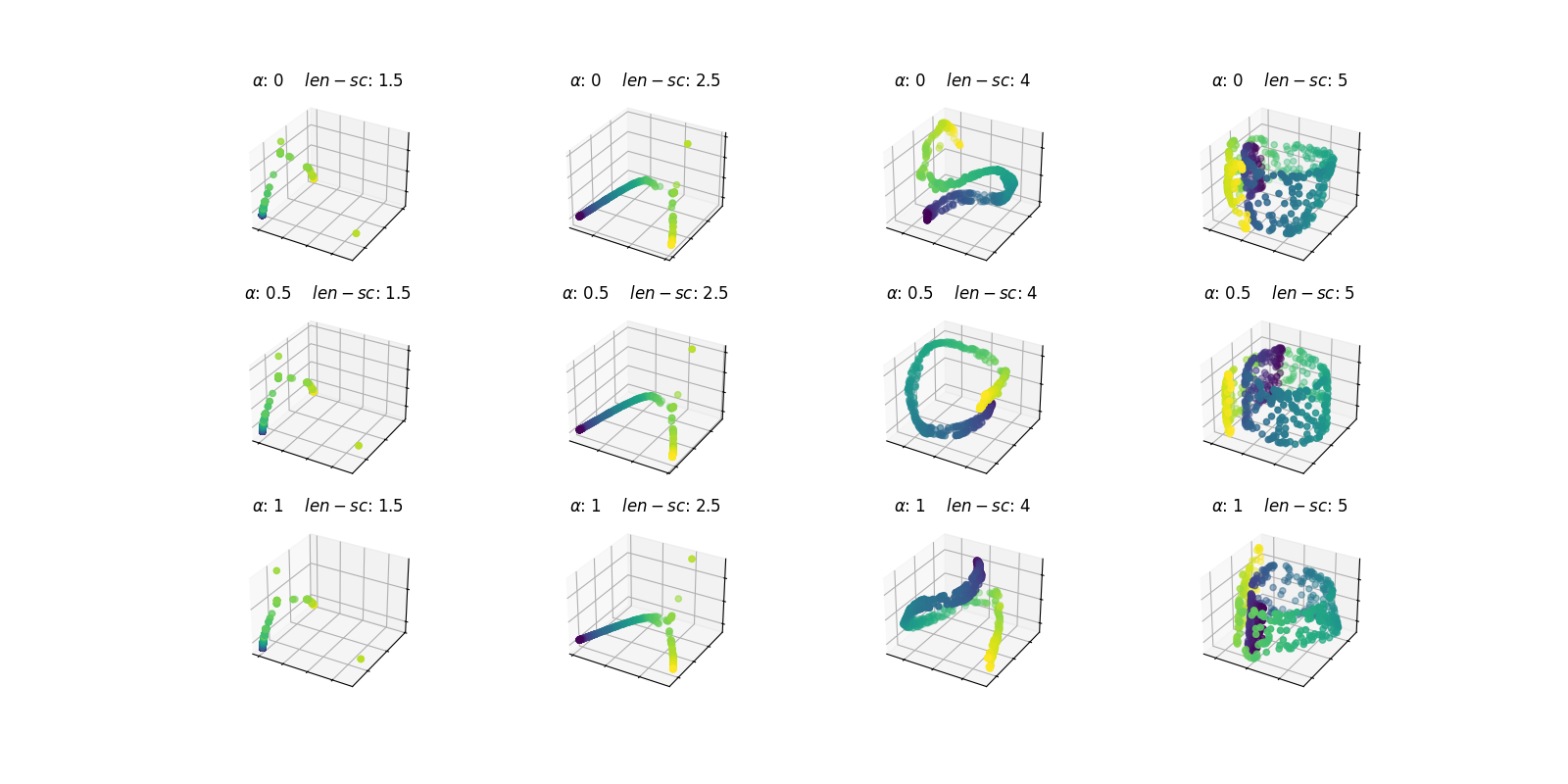
Now, the FDM method will be applied for different values of the parameters, again in the form of a grid search. Note that the diffusion coordinates will now consist of three components.

alpha_set = [0, 0.5, 1]
length_scale_set = [1.5, 2.5, 4, 5]
param_grid = product(alpha_set, length_scale_set)

fig, axes = plt.subplots(
    len(alpha_set),
    len(length_scale_set),
    figsize=(16, 8),
    subplot_kw={"projection": "3d"},
)

for (alpha, length_scale), ax in zip(param_grid, axes.ravel(), strict=True):

    fdm = DiffusionMap(
        n_components=3,
        kernel=Gaussian(length_scale=length_scale),
        alpha=alpha,
        n_steps=1,
    )
    embedding = fdm.fit_transform(fd_swiss)

    ax.scatter(embedding[:, 0], embedding[:, 1], embedding[:, 2], c=y)
    ax.set_xticklabels([])
    ax.set_yticklabels([])
    ax.set_zticklabels([])
    ax.set_title(f"$\\alpha$: {alpha}    $len-sc$: {length_scale}")

plt.show()

Let’s take a closer look at the resulting embedding for a value of length_scale and alpha equal to 2.5 and 0, respectively.

alpha, length_scale = 0, 2.5
fdm = DiffusionMap(
    n_components=3,
    kernel=Gaussian(length_scale=length_scale),
    alpha=alpha,
    n_steps=1,
)
embedding = fdm.fit_transform(fd_swiss)

fig = plt.figure()
ax = fig.add_subplot(111, projection="3d")
ax.scatter(embedding[:, 0], embedding[:, 1], embedding[:, 2], c=y)
ax.set_title(
    "Diffusion coordinates for \n"
    f"$\\alpha$: {alpha}    $len-sc$: {length_scale}",
)
plt.show()

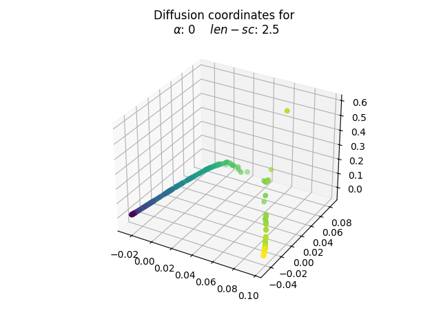
The election of the optimal parameters is relative to the problem at hand. The goal behind choosing values of length_scale equal to 2.5 and alpha equal to 0 is to obtain a unrolled transformation to the Swiss roll. Note that in the roll there are pairs of points whose euclidean distance is small but whose shortest path contained in the manifold is significantly larger, since it must complete an entire loop.

In this sense, the process happens to have taken into account the shortest path distance rather than the euclidean one. Thus, one may argue that the topological nature of the data has been respected. This new diffusion coordinates could be useful to gain more insights into the initial data through further analysis.

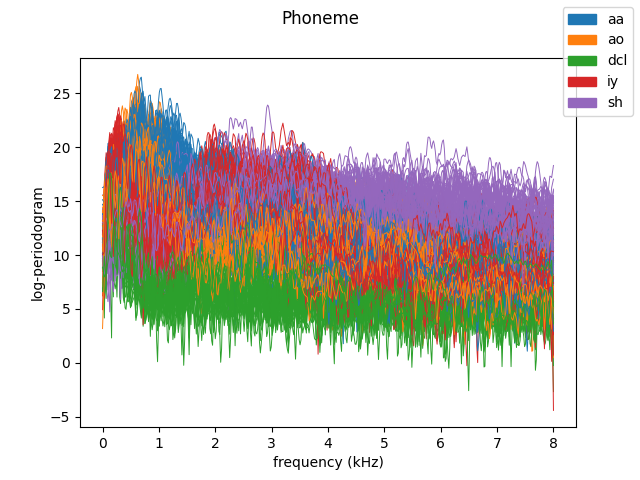
Real dataset: phoneme

The aim of this section is to provide an example of application of the FDM method to a non-synthetic dataset. Below is an example of execution using the phoneme dataset, a dataset consisting of the computed log-periodogram for five distinct phonemes coming from recorded male speech from the TIMIT database.

from skfda.datasets import fetch_phoneme

n_samples = 300
colors = ["C0", "C1", "C2", "C3", "C4"]
group_names = ["aa", "ao", "dcl", "iy", "sh"]

# Fetch phoneme dataset
fd_phoneme, y = fetch_phoneme(return_X_y=True)
fd_phoneme, y = fd_phoneme[:n_samples], y[:n_samples]
fd_phoneme.plot(
    linewidth=0.7,
    group=y,
    group_colors=colors,
    group_names=group_names,
    legend=True,
)
plt.show()

The resulting diffusion coordinates in three dimensions will be plotted, using different views to better understand the plot.

cmap = ListedColormap(colors)
alpha, length_scale = 1, 10
fdm = DiffusionMap(
    n_components=3,
    kernel=Gaussian(length_scale=length_scale),
    alpha=alpha,
    n_steps=1,
)
diffusion_coord = fdm.fit_transform(fd_phoneme)

# Plot three views of the diffusion coordinates
view_points = [(30, 70), (28, 0), (10, -120)]

fig, axes = plt.subplots(
    1, len(view_points), figsize=(18, 6), subplot_kw={"projection": "3d"},
)

for view, ax in zip(view_points, axes.ravel(), strict=True):
    ax.scatter(
        diffusion_coord[:, 0],
        diffusion_coord[:, 1],
        diffusion_coord[:, 2],
        c=y,
        cmap=cmap,
    )
    ax.view_init(*view)
    ax.set_title(f"View {view}", fontsize=26)
plt.show()

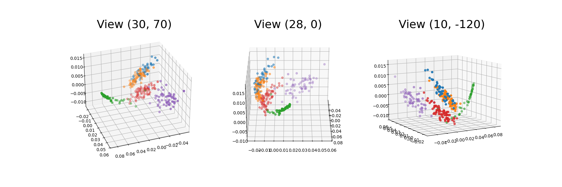
We can see that the diffusion coordinates for the different phonemes have been clustered in the 3D space. This representation enables a more clear separation of the data into the different phoneme groups. In this way, the phonemes groups that are similar to each other, namely /aa/ and /ao/ are closer in the space. In fact, these two groups partly overlap (orange and blue).

References

[1]

M. Barroso, C. M. Alaíz, J. L. Torrecilla, and A. Fernández. Functional diffusion maps. Statistics and Computing, 34(1):22, 2023. URL: https://doi.org/10.1007/s11222-023-10332-1, doi:10.1007/s11222-023-10332-1.